SpatAn 2: Exercise B

In the last exercise, you had your first experience with raster data. We first rasterised a vector dataset. However, we often work with spatial data that has already been captured in raster format.

Task 1

In this exercise, we will continue to work with terra to show how we can import, visualise and further process a raster dataset. In your data you will find a dataset called dhm250m.tif, which represents the “Digital Elevation Model” (DHM) of the Canton of Schwyz. Execute the specified code.

library("terra")

Import your raster with the rast() function

dhm_schwyz <- rast("datasets/rauman/dhm250m.tif")

You will get some important metadata about the raster data when you enter the variable name in the console.

## class       : SpatRaster 
## dimensions  : 150, 186, 1  (nrow, ncol, nlyr)
## resolution  : 250, 250  (x, y)
## extent      : 2672175, 2718675, 1193658, 1231158  (xmin, xmax, ymin, ymax)
## coord. ref. : CH1903+ / LV95 (EPSG:2056) 
## source      : dhm250m.tif 
## name        :   dhm250m 
## min value   :  389.1618 
## max value   : 2850.0203

To get a quick overview of a raster record, we can simply use the plot() function.

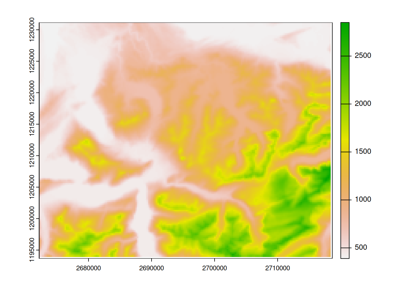
Unfortunately, using raster data in ggplot is not very easy. Since ggplot() is a universal plot framework, we quickly reach the limits of what is possible when we create something as special as a map. Plot allows us to work very quickly, but again, it has its limits.

For this reason, we will introduce a new plot framework that specialises in maps and is built in a very similar design to ggplot: tmap. Load this package into your session now:

library("tmap")

Just like ggplot(), tmap is based on the idea of “layers” connected by a +. Each level has two components:

• a dataset component that is always tm_shape(dataset) (replace dataset with your variable)
• a geometry component that describes how the previous tm_shape() should be visualised. This can be tm_dots() for points, tm_polygons() for polygons, tm_lines() for lines, etc. For single band raster (which is the case with dhm_ schwyz), use tm_raster()

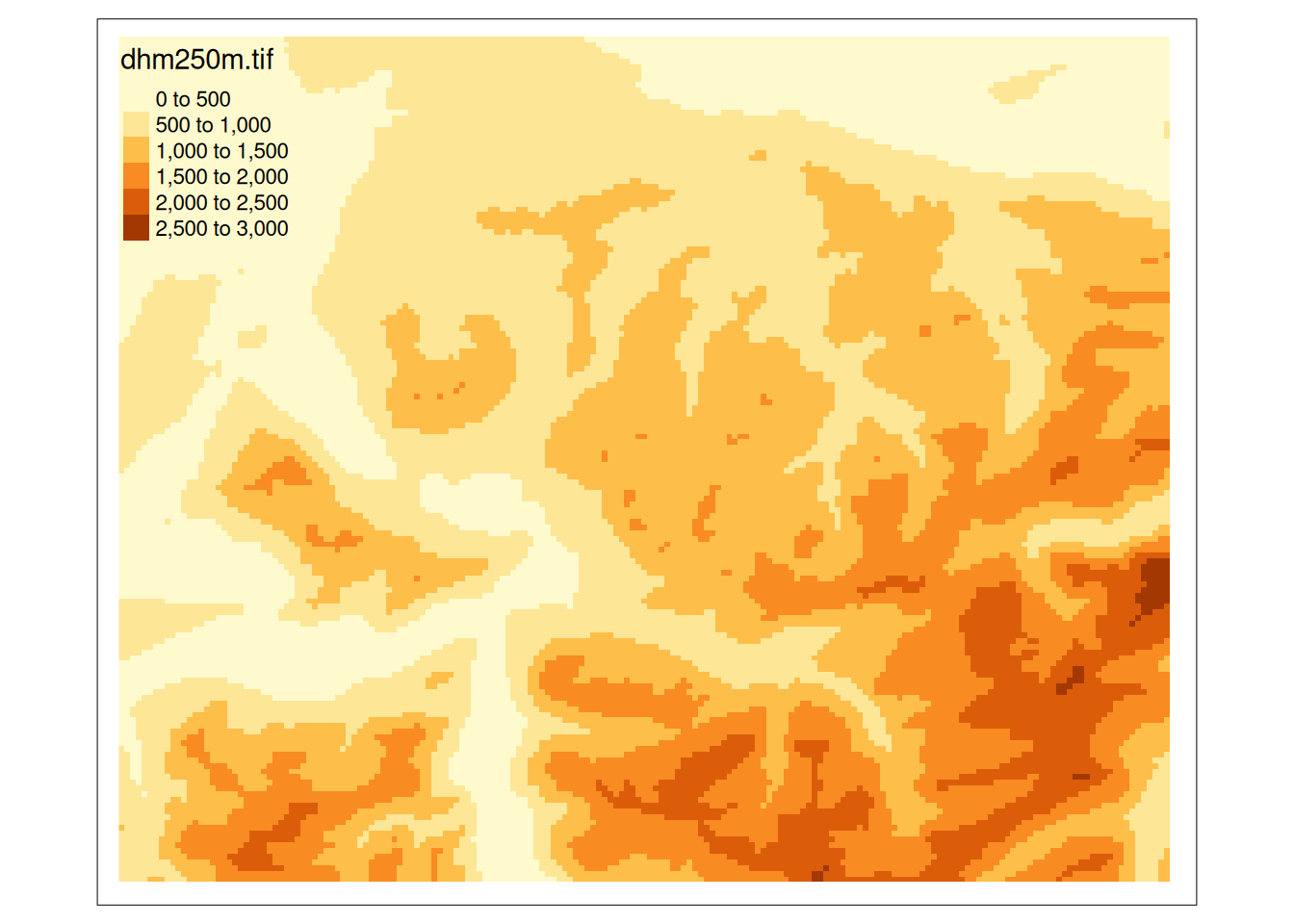
Note that tm_shape() and tm_raster() (in this case) cannot exist without each other.

If you consult?tm_raster, you will see a variety of options that you can how your data is visualised. For example, the default style of tm_raster() creates “bins” with a discrete colour gamut. We can override this with style = "cont".

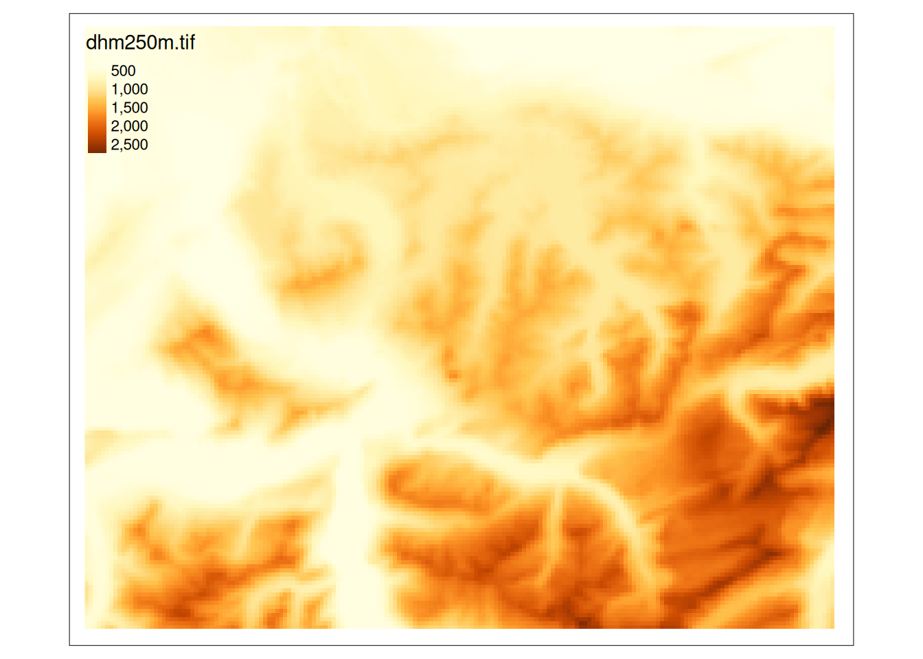
That should look appropriate, but maybe we want to change the default colour palette. Fortunately, this is much easier in tmap than in ggplot2. To view the available palettes, enter tmaptools ::palette_explorer() or RColorBrewer:: display.brewer.all() in the console (for the former, you may need to install additional packages, e.g. shinyjs).

One of tmap’s great strengths is the fact that both static and interactive plots can be created with the same command. For this, you need to change the mode from static to interactive.

Task 2

Using terra, we can run a variety of raster operations on our elevation model. A classic raster operation is the calculation of a slope’s incline (“slope”) or its orientation (“aspect”). Use the terrain() function from terra to calculate the slope inclination and orientation. Visualise the results.

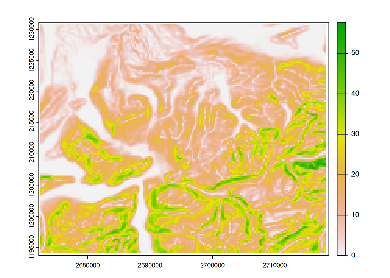
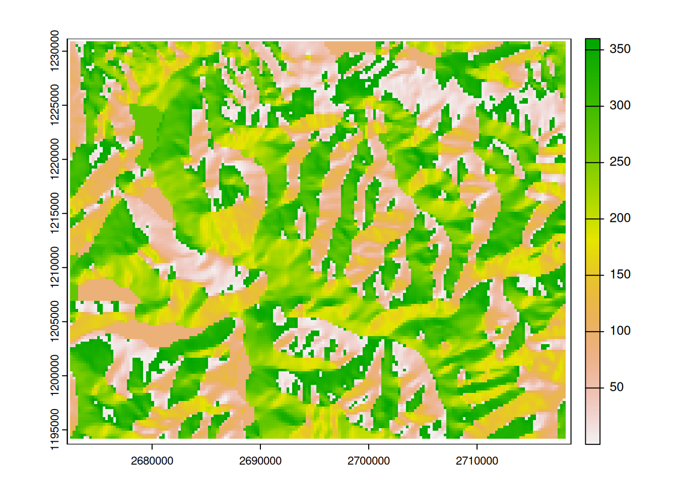
Note

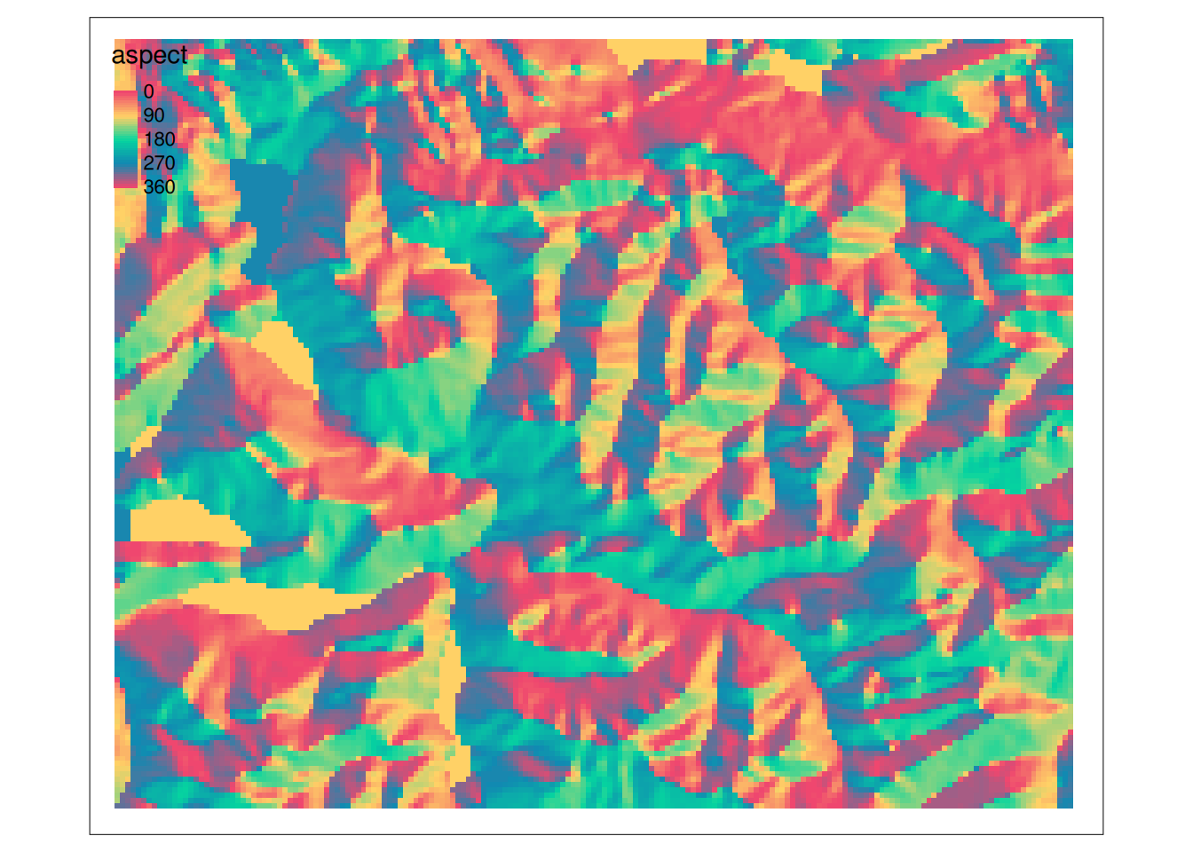
“aspect” is a value that ranges from 0 to 360. In classic pallets, the two extreme values (in this case 0 and 360) are far apart in terms of colour. In aspect, however, these should be close together (since an orientation of 1° is only 2 degrees away from an orientation of 359°). To take this fact into account, we can create our own colour palette, where the first colour is repeated.

Task 3

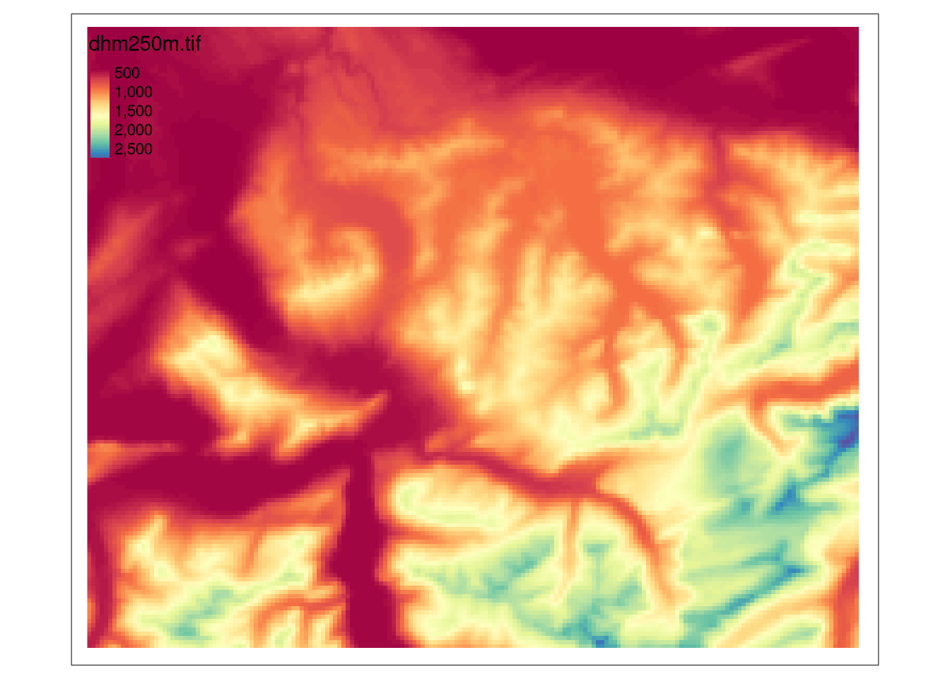
Using slope incline and orientation, we can calculate a hill shading effect. Hill shading refers to the shadow cast on the surface model and is calculated at a given angle of the sun (height and azimuth). The typical angle is 45° above the horizon and 315° from the northwest.

To create a hill shading effect, first calculate slope and aspect of dhm_schwyz, just like in the previous task, but make sure that the unit corresponds to the radians. Use these two objects in the shade() function to calculate the hill shade. Then visualise the output with plot or tmap.

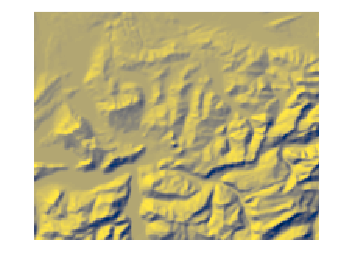
Use tmap for this visualisation along side the cividis colour palette