SpatAn 2: Exercise A

Please download the data for todays exercise here: SpatAn2.

In the last exercise, we performed a spatial join between trees and meadows to find out whether a tree is in a meadow or not using data from the Grüental campus (gruental.gpkg)

Today we will go a step further and try to answer the following question: How much meadow is there within 20 metres of each tree?

To do this, load the required libraries and records into your session. Explore the data and visualize it spatially.

library("dplyr")
library("sf")
library("ggplot2")

meadows <- read_sf("datasets/rauman/gruental.gpkg", "wiesen")
trees <- read_sf("datasets/rauman/gruental.gpkg", "baeume")

In order to simplify the exercise a little, we will only work with 10 trees at first. Use the code below to randomly select 10 trees. If you use the same “seed” as we have(set.seed(100)), you should also “coincidentally” have the same trees as me.

set.seed(100)
trees_sample <- sample_n(trees, 10)

ggplot() +
  geom_sf(data = meadows) +
  geom_sf(data = trees_sample)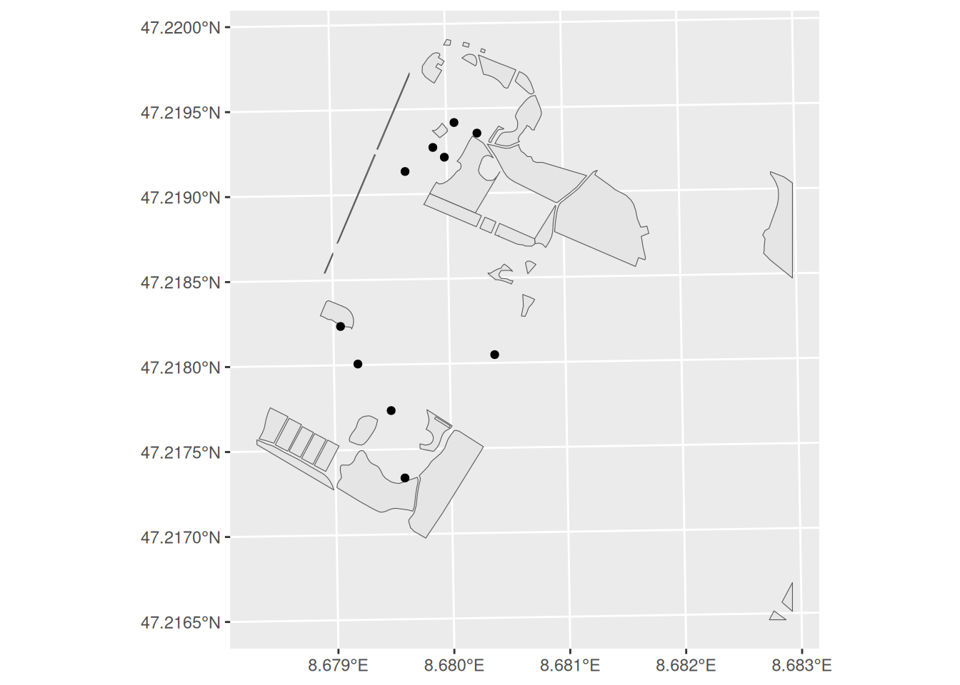

Task 1

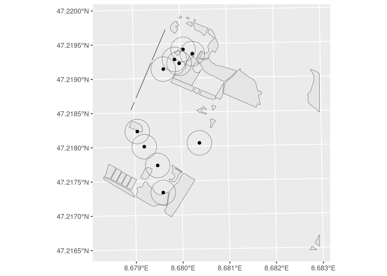
As a first step, we need to apply a 20m buffer to each tree. Use st_buffer to save the output as trees_20m. Now take a close look at trees_20m. What type of geometry does it now represent?

Figure 23.1: Trees are displayed as points with a 20m buffer. Meadows are displayed in the background.

Task 2

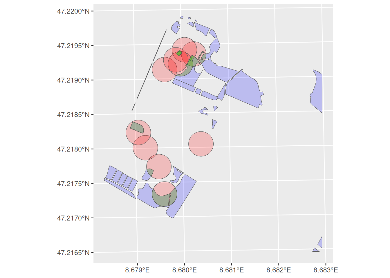
Now calculate the intersection of trees_20m and meadows with the st_intersection function and save the output as trees_meadows. Next explore trees_meadows. What happened? Check the number of rows per record. Have they changed? If so, why?

Task 3

Now calculate the area per geometry with the st_area() function. Save the output in a new column called trees_meadows (e.g. with the name meadow_area). Tip: Convert the output from st_area() to a numeric vector with as.numeric().

Task 4 (Optional)

Now calculate the meadow_share from meadow_area. Tip: The circular area of \(r^2\times \pi\) is 100%, whereas in our case, $r = $20.

Then transfer the calculated proportional values to the trees dataset with a left_ join() between trees and trees_meadows. Which column would be suitable for this join? Note: Use st_drop_geometry() to remove the geometry column in trees_meadows before joining.

Figure 23.2: After this exercise, you can visualise the results like this.

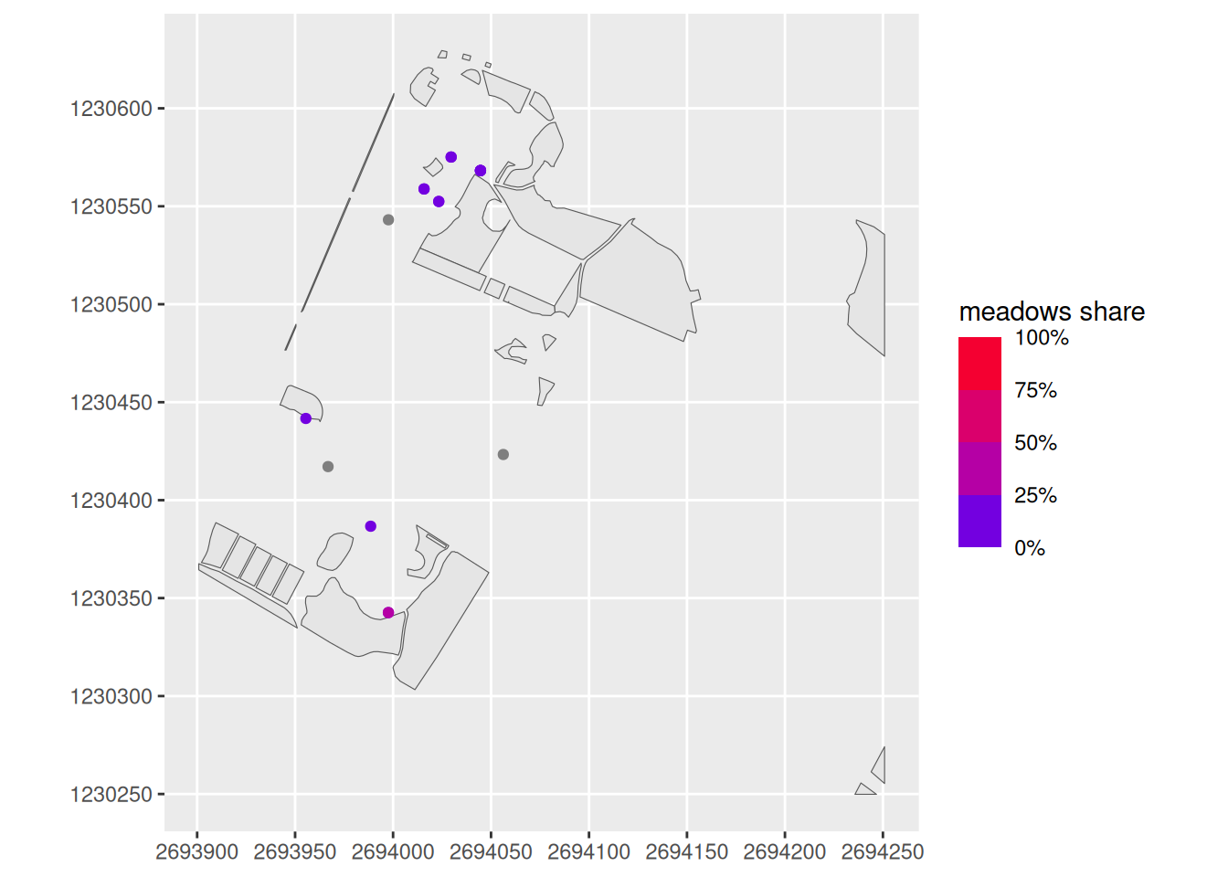
Task 5

By now you have performed a few vector operations such as st_buffer() and st_intersection() and st_area(). However, certain questions are better answered using the raster format. For example, if we want to know how far the nearest tree is for each point in the room, this can be better represented in a raster.

However, before we can answer that question, we have to convert the vector data set into a raster data set. To do this, a raster “template” is needed so that R knows roughly what the raster output should look like.

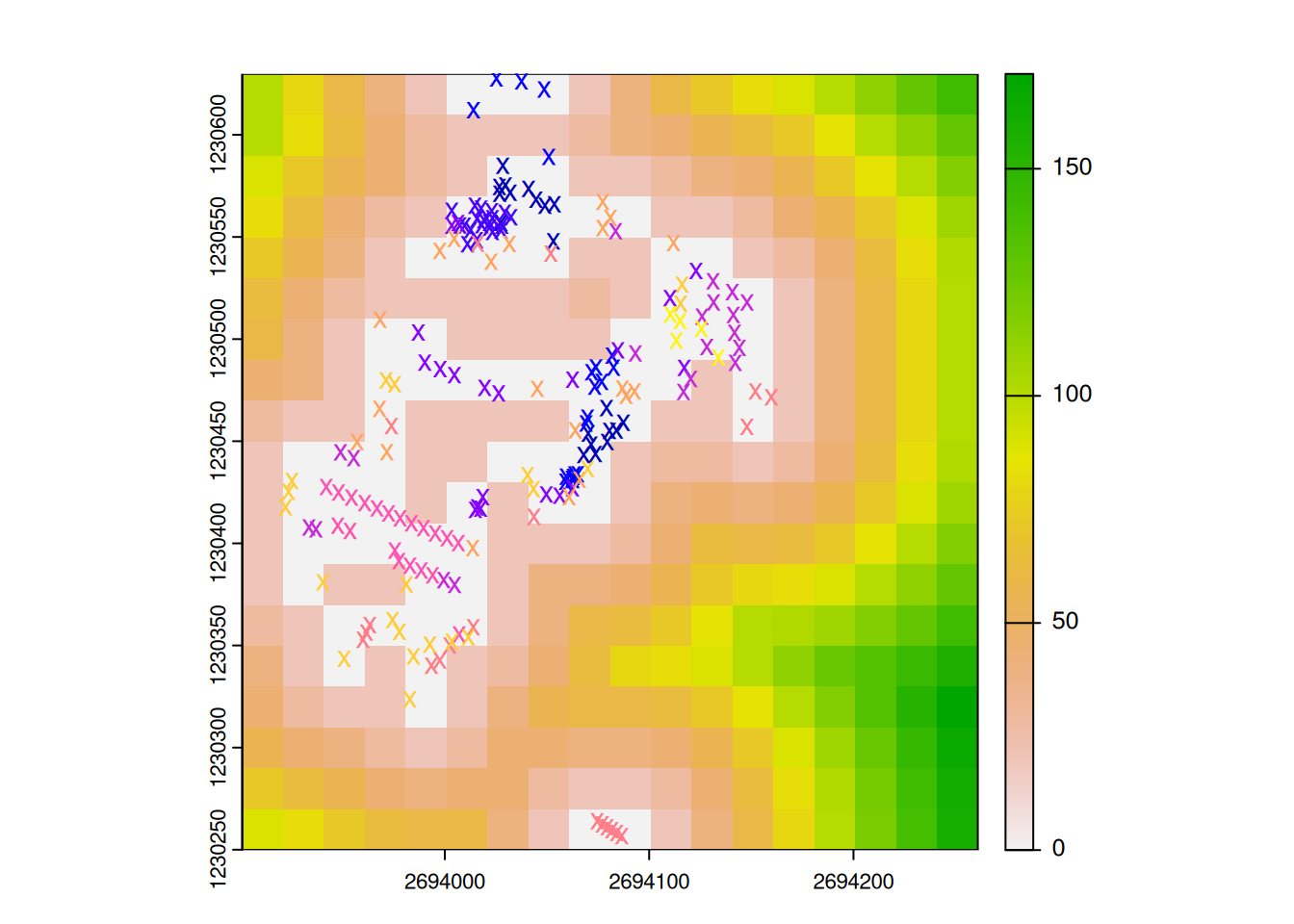
The difference between raster and vector can be shown very vividly if the two data sets are stored one on top of the other.

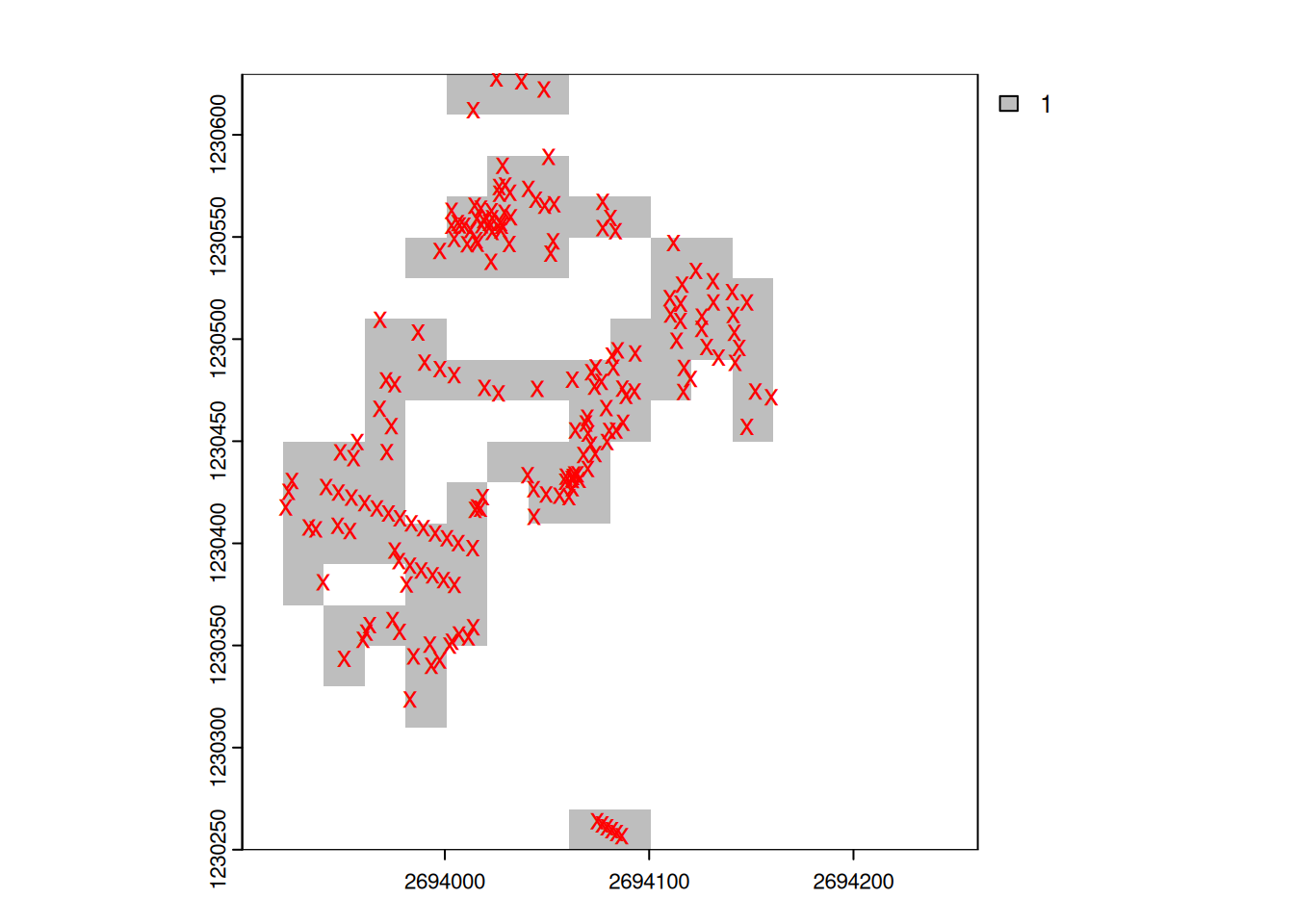
we can now use the function distance() with trees_rast to calculate the distance to each tree: