Prepro 3: Exercise

Task 1

You have a dataset, sensors_long.csv, with temperature values from three different sensors. Import it as a csv into R (as sensors_long).

Reformat the datetime column to POSIXct. Use the as.POSIXct function (read it in using?strftime()) to determine the specific format (the template).

library("readr")

sensors_long <- read_delim("datasets/prepro/sensors_long.csv", ",")

Task 2

Group sensors_long according to the column name where the sensor information is contained, using the function group_by, and calculate the average temperature for each sensor (summarise). Note: Both functions are part of the dplyr package.

The output will look like this:

library("dplyr")

sensors_long |>
  group_by(name) |>
  summarise(temp_mean = mean(value, na.rm = TRUE))
## # A tibble: 3 × 2
##   name    temp_mean
##   <chr>       <dbl>
## 1 sensor1      14.7
## 2 sensor2      12.0
## 3 sensor3      14.4

Task 3

Create a new convenience variable, month, for sensors_long (Tip: use the month function from lubridate). Now group by month and sensor and calculate the mean temperature.

library("lubridate")

sensors_long |>
  mutate(month = month(Datetime)) |>
  group_by(month, name) |>
  summarise(temp_mean = mean(value, na.rm = TRUE))
## # A tibble: 6 × 3
## # Groups:   month [2]
##   month name    temp_mean
##   <dbl> <chr>       <dbl>
## 1    10 sensor1     14.7 
## 2    10 sensor2     12.7 
## 3    10 sensor3     14.4 
## 4    11 sensor1    NaN   
## 5    11 sensor2      8.87
## 6    11 sensor3    NaN

Task 4

Now import the weather.csv dataset (source MeteoSwiss) with the correct column types (time as POSIXct, tre200h0 as double). You can download the file from moodle if you havent done so yet.

weather <- read_delim("datasets/prepro/weather.csv")


weather$time2 <- weather$time |> 
  as.character() |> 
  as.POSIXct(format = "%Y%m%d%H", tz = "UTC")
  

weather$time <- weather$time2
weather$time2 <- NULL

Task 5

Now create a convenience variable for the calendar week for each measurement (lubridate::isoweek). Then calculate the average temperature value for each calendar week.

weather_summary <- weather |>
  mutate(week = isoweek(time)) |>
  group_by(week) |>
  summarise(
    temp_mean = mean(tre200h0, na.rm = TRUE)
  )

Next, you can visualise the result using the following function:

plot(weather_summary$week, weather_summary$temp_mean, type = "l")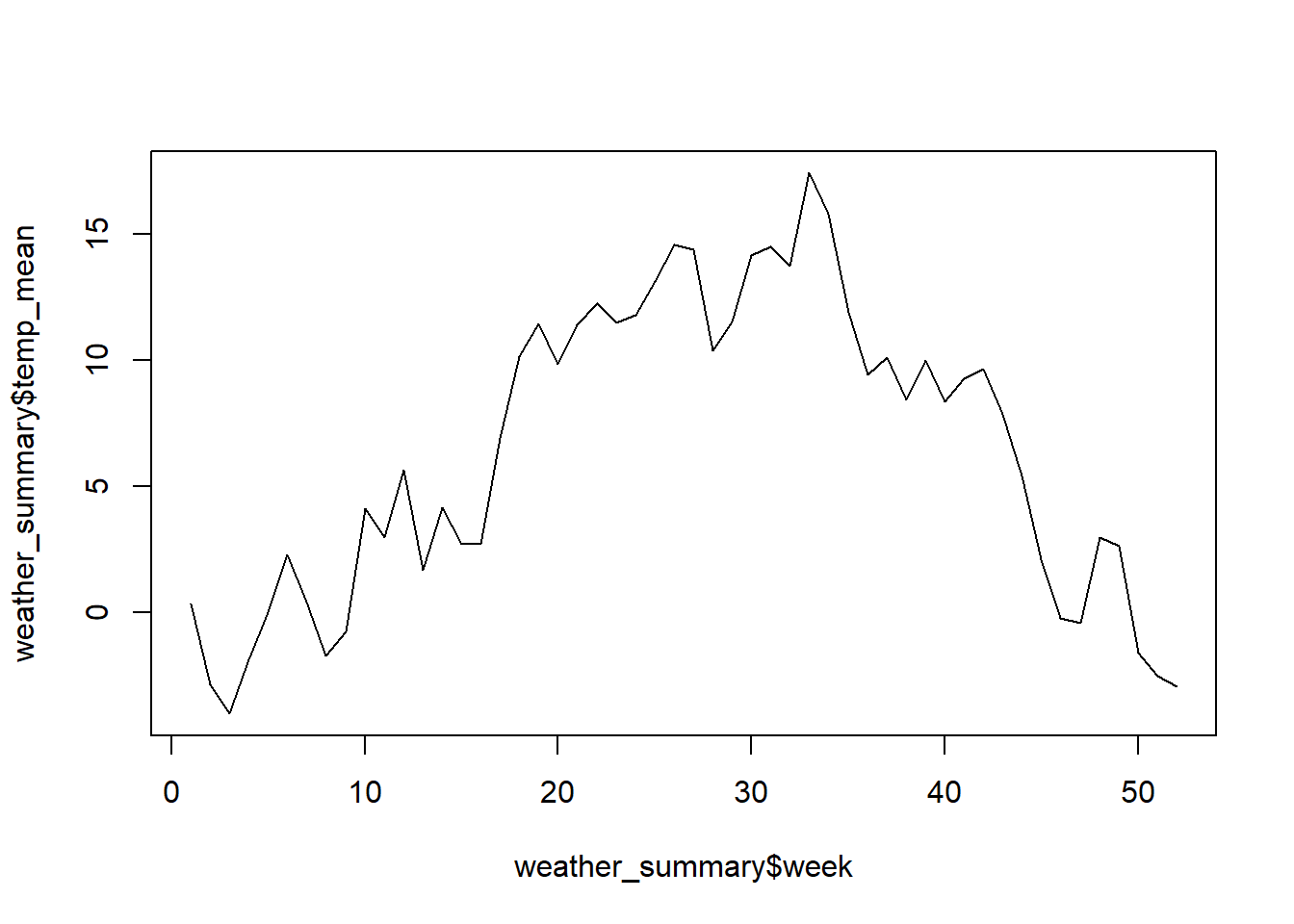

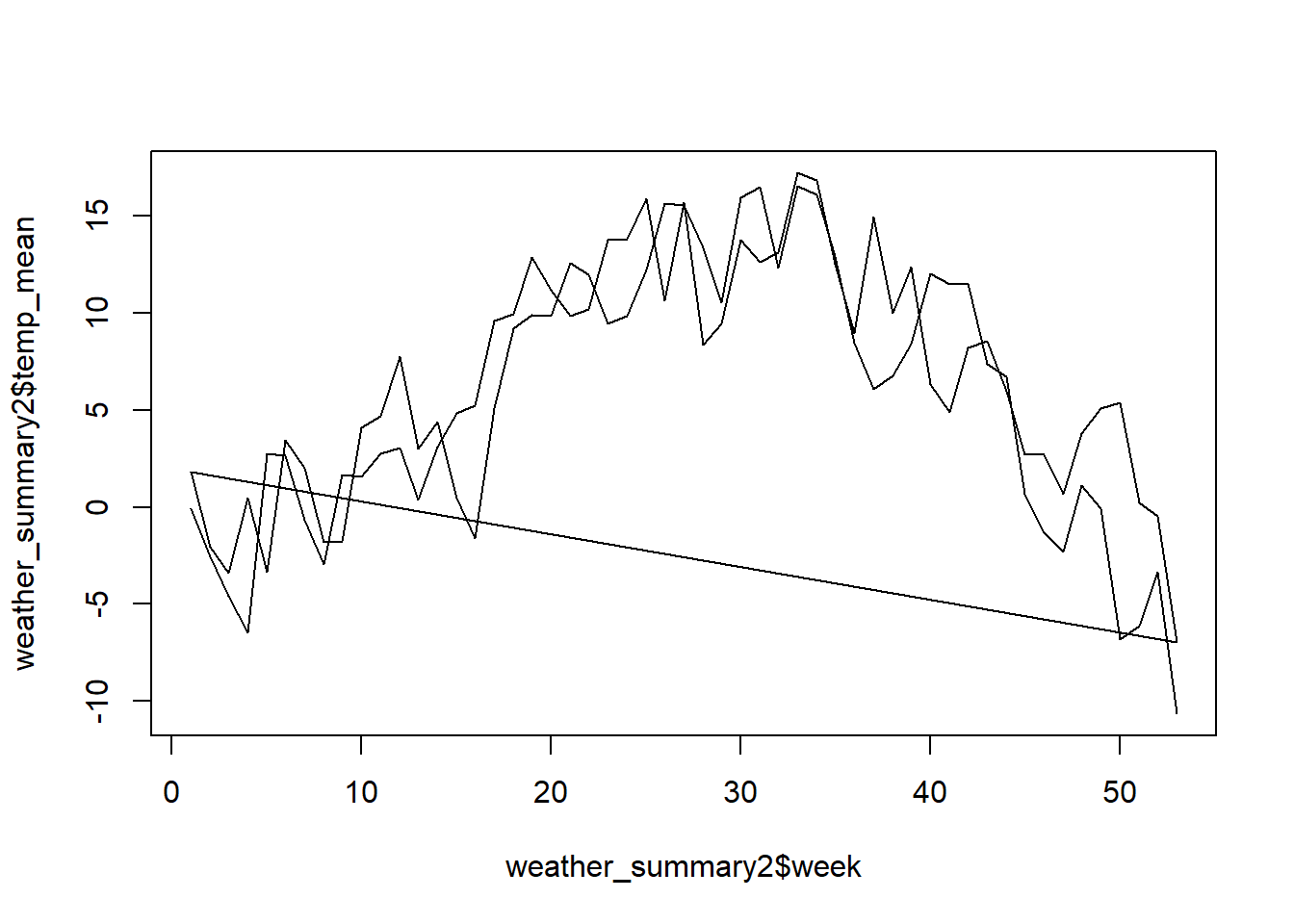
Task 6

In the previous task, we calculated the average temperature per calendar week over all years (2000 and 2001). However, if we want to compare the years with each other, we have to create the year as an additional convenience variable and group it accordingly. Try this with the weather data and then visualise the output.

weather_summary2 <- weather |>
  mutate(
    week = week(time),
    year = year(time)
    ) |>
  group_by(year, week) |>
  summarise(
    temp_mean = mean(tre200h0, na.rm = TRUE)
  )

plot(weather_summary2$week, weather_summary2$temp_mean, type = "l")

Figure 9.1: Base plot does not like long tables and makes a continuous line out of the two years